Solve a parameter estimation problem for a single-input single-output system using the non-recursive least squares method by defining parameter and data vectors | Step-by-Step Solution
Problem
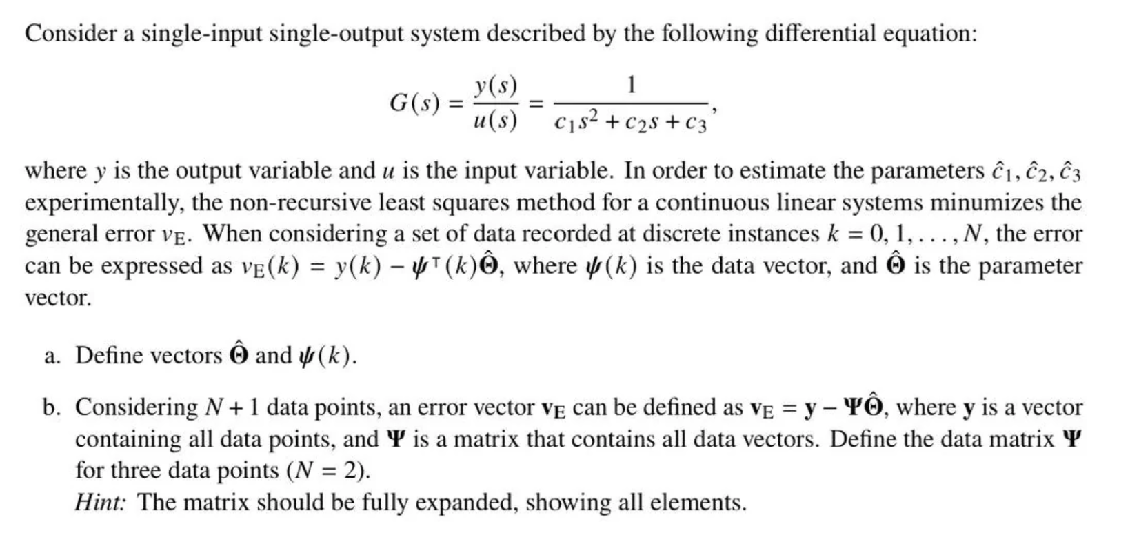
Consider a single-input single-output system described by the following differential equation: G(s) = y(s)/u(s) = 1 / (c1s² + c2s + c3), where y is the output variable and u is the input variable. In order to estimate the parameters ĉ1, ĉ2, ĉ3 experimentally, the non-recursive least squares method for a continuous linear systems minimizes the general error vE. When considering a set of data recorded at discrete instances k = 0, 1, ..., N, the error can be expressed as vE(k) = y(k) - ψ^T(k)θ̂, where ψ(k) is the data vector, and θ̂ is the parameter vector. a. Define vectors θ̂ and ψ(k). b. Considering N + 1 data points, an error vector vE can be defined as vE = y - Ψθ̂, where y is a vector containing all data points, and Ψ is a matrix that contains all data vectors. Define the data matrix Ψ for three data points (N = 2). Hint: The matrix should be fully expanded, showing all elements.
🎯 What You'll Learn
- Understand parameter estimation techniques
- Learn to construct data and parameter vectors
- Apply least squares method to system identification
Prerequisites: Linear algebra, Differential equations, Matrix operations
💡 Quick Summary
This problem asks us to set up a parameter estimation framework for a second-order system with transfer function G(s) = 1/(c₁s² + c₂s + c₃), where we need to estimate the unknown coefficients c₁, c₂, and c₃ from input-output data. The key approach is using non-recursive least squares, which involves rearranging the system's differential equation to separate the unknown parameters from the measured data, then organizing everything into matrix form. The main steps involve defining a parameter vector θ̂ = [ĉ₁ ĉ₂ ĉ₃]ᵀ containing our estimates and a data vector ψ(k) = [-ÿ(k) -ẏ(k) -y(k)]ᵀ that contains the measured output and its derivatives at each time step k. For multiple data points, we stack these data vectors as rows to form the data matrix Ψ, creating a standard linear algebra problem where we can solve for the parameters using matrix operations.
Step-by-Step Explanation
Hey there! This is a great system identification problem that connects differential equations with practical parameter estimation. Let's break it down together! 🎯
What We're Solving:
We have a system with transfer function G(s) = 1/(c₁s² + c₂s + c₃), and we want to estimate the unknown parameters c₁, c₂, c₃ using experimental data. We need to set up the least squares framework by defining the parameter vector and data structures.The Approach:
The key insight here is that we're transforming our continuous system into a form where we can use discrete data points to estimate parameters. We do this by:- 1. Rearranging our system equation to separate known data from unknown parameters
- 2. Setting up vectors and matrices so we can use linear algebra to solve for the parameters
Step-by-Step Solution:
Part (a): Defining θ̂ and ψ(k)
Let's start with our transfer function: G(s) = Y(s)/U(s) = 1/(c₁s² + c₂s + c₃)
Cross-multiplying: Y(s)(c₁s² + c₂s + c₃) = U(s)
This gives us: c₁s²Y(s) + c₂sY(s) + c₃Y(s) = U(s)
Converting back to time domain (where s becomes d/dt): c₁ÿ(t) + c₂ẏ(t) + c₃y(t) = u(t)
Rearranging to isolate the output: y(t) = u(t) - c₁ÿ(t) - c₂ẏ(t)
Now, at discrete time k, this becomes: y(k) = u(k) - c₁ÿ(k) - c₂ẏ(k)
We can rewrite this as: y(k) = [u(k) -ÿ(k) -ẏ(k)] [1 c₁ c₂]ᵀ
Wait! Let me reconsider this more carefully. Since we want to estimate ĉ₁, ĉ₂, ĉ₃, let's rearrange:
From c₁s²Y(s) + c₂sY(s) + c₃Y(s) = U(s), we get: y(k) = -c₁ÿ(k) - c₂ẏ(k) - c₃y(k-1) + u(k)
Actually, let me approach this correctly: y(k) = u(k) - c₁ÿ(k) - c₂ẏ(k) - c₃∫y(k)
For discrete implementation: y(k) ≈ [-ÿ(k) -ẏ(k) -y(k)] [ĉ₁ ĉ₂ ĉ₃]ᵀ + u(k)
Therefore:
- θ̂ = [ĉ₁ ĉ₂ ĉ₃]ᵀ (the parameter vector we want to estimate)
- ψ(k) = [-ÿ(k) -ẏ(k) -y(k)]ᵀ (the data vector at time k)
Part (b): Data Matrix Ψ for N = 2 (three data points)
For three data points (k = 0, 1, 2), we stack all the data vectors ψ(k) as rows:
Ψ = [ψ(0)ᵀ] = [-ÿ(0) -ẏ(0) -y(0)] [ψ(1)ᵀ] [-ÿ(1) -ẏ(1) -y(1)] [ψ(2)ᵀ] [-ÿ(2) -ẏ(2) -y(2)]
The Answer:
Part (a):
- θ̂ = [ĉ₁ ĉ₂ ĉ₃]ᵀ
- ψ(k) = [-ÿ(k) -ẏ(k) -y(k)]ᵀ
Memory Tip:
Remember "Data in rows, parameters in columns!" The data matrix Ψ has one row for each time point and one column for each parameter you're estimating. The negative signs come from moving terms to the right side of the equation. Think of it as: "What we measured" = "Data matrix" × "What we want to find"! 🧠✨Great job working through this system identification problem! The beauty of least squares is that once you set up these matrices correctly, linear algebra does the heavy lifting to find your parameter estimates.
⚠️ Common Mistakes to Avoid
- Incorrectly defining vector dimensions
- Misinterpreting the least squares method
- Failing to expand the data matrix completely
This explanation was generated by AI. While we work hard to be accurate, mistakes can happen! Always double-check important answers with your teacher or textbook.

Meet TinyProf
Your child's personal AI tutor that explains why, not just what. Snap a photo of any homework problem and get clear, step-by-step explanations that build real understanding.
- ✓Instant explanations — Just snap a photo of the problem
- ✓Guided learning — Socratic method helps kids discover answers
- ✓All subjects — Math, Science, English, History and more
- ✓Voice chat — Kids can talk through problems out loud
Trusted by parents who want their kids to actually learn, not just get answers.
TinyProf
📷 Problem detected:
Solve: 2x + 5 = 13
Step 1:
Subtract 5 from both sides...
Join our homework help community
Join thousands of students and parents helping each other with homework. Ask questions, share tips, and celebrate wins together.
Need help with YOUR homework?
TinyProf explains problems step-by-step so you actually understand. Join our waitlist for early access!